How Do Computers Store Audio?
Prerequisites
Some basic knowledge of the following is assumed:
-
Basic math knowledge
Continuous vs Discrete Data
First off, though, we need to cover some terminology, so that the reasoning for some concepts we’ll discuss later on will be clear.
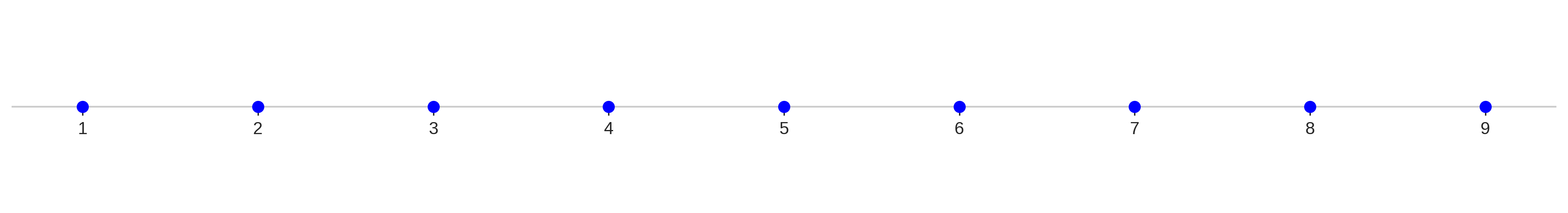
If I asked you to name how many integers (numbers without a decimal) are greater than 0 and less than 10, what would you say? The logical answer is, of course, 9: 1, 2, 3, 4, 5, 6, 7, 8, and 9 are all greater than 0 and less than 10, giving a grand total of 9 numbers.
Now, if I asked you to mark these values on a number line, you might end up with something like this:
However, what if I said numbers includes decimal numbers? Well there’s 0.1, 0.01, 0.001, 0.00001, … Turns out, there are an infinite amount of numbers greater than 0 and less than 10.
If you had to mark these on a number line…well, you couldn’t. There’s an infinite number of points that would have to be marked. Instead, it’s generally represented as just, well, a line:
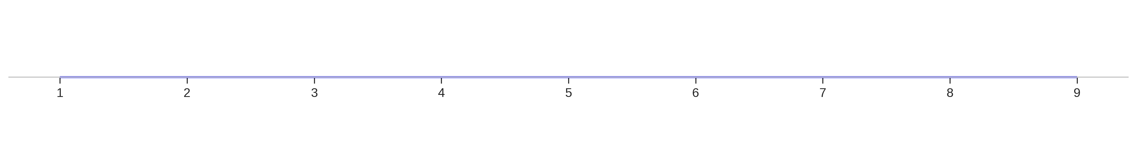
This line represents what we’d call continuous data: the data contains an infinite number of points along its range. This contrasts to the first example, which consisted of discrete data points.
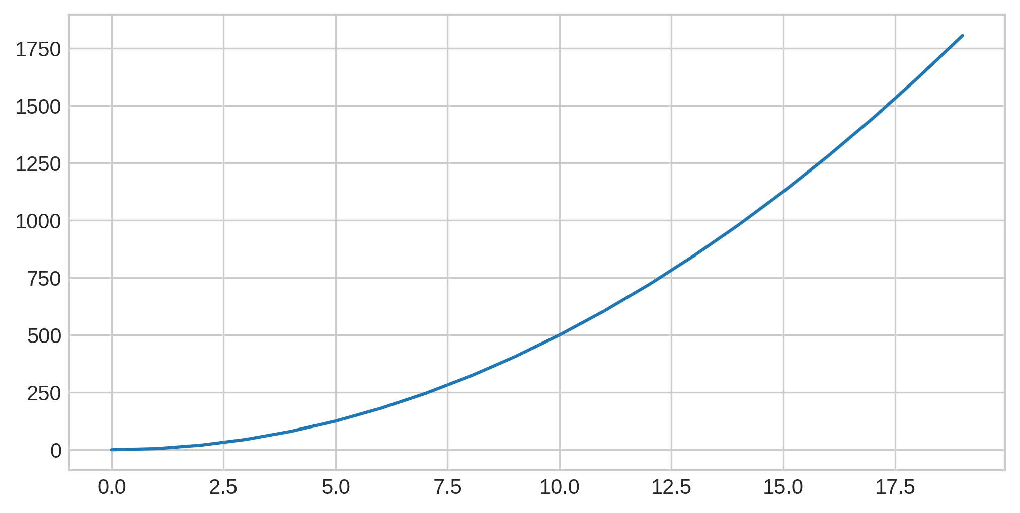
Let’s level things up a bit. This graph shows a continuous line:
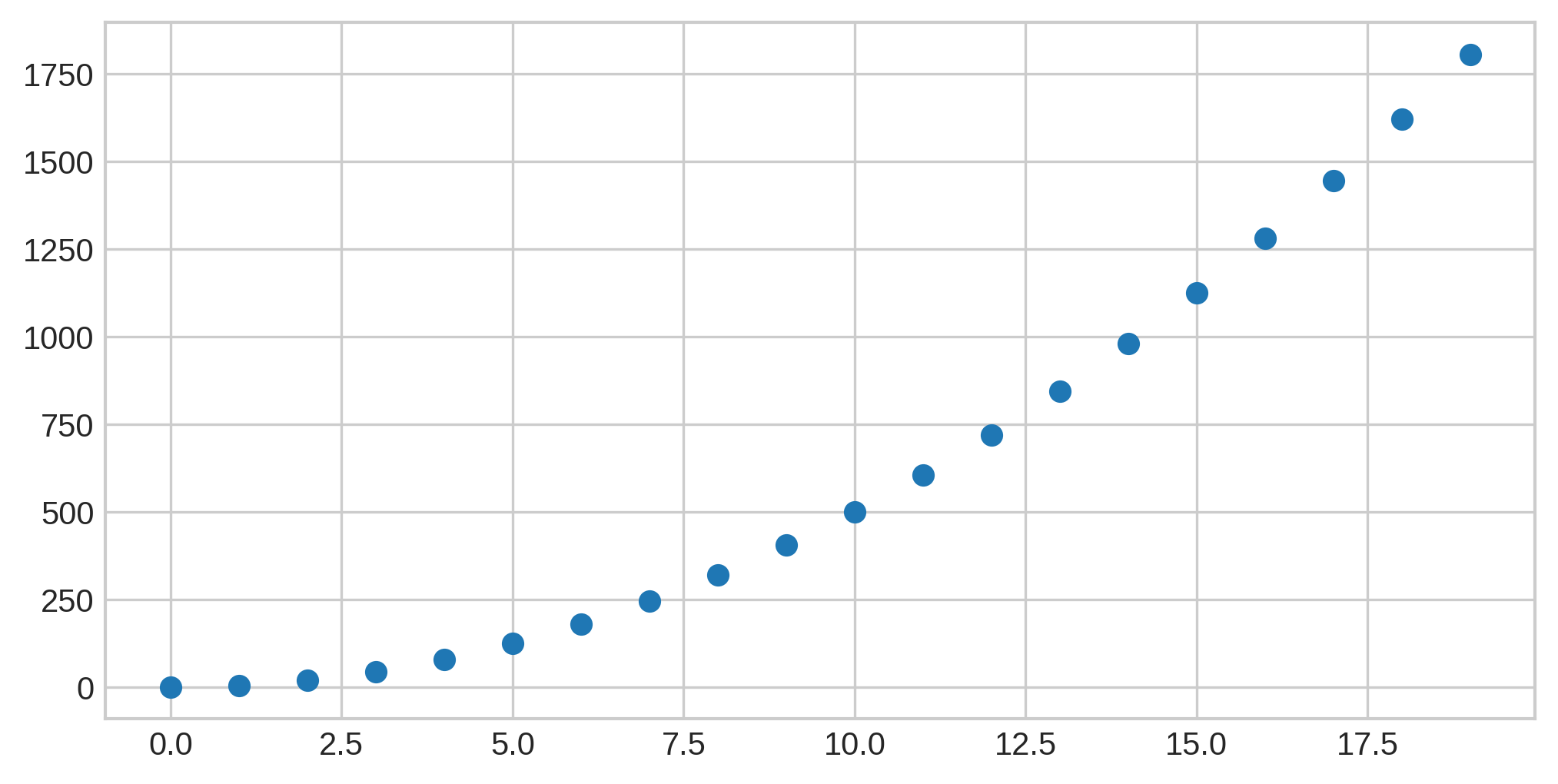
and this graph shows discrete data points:
Sound Waves
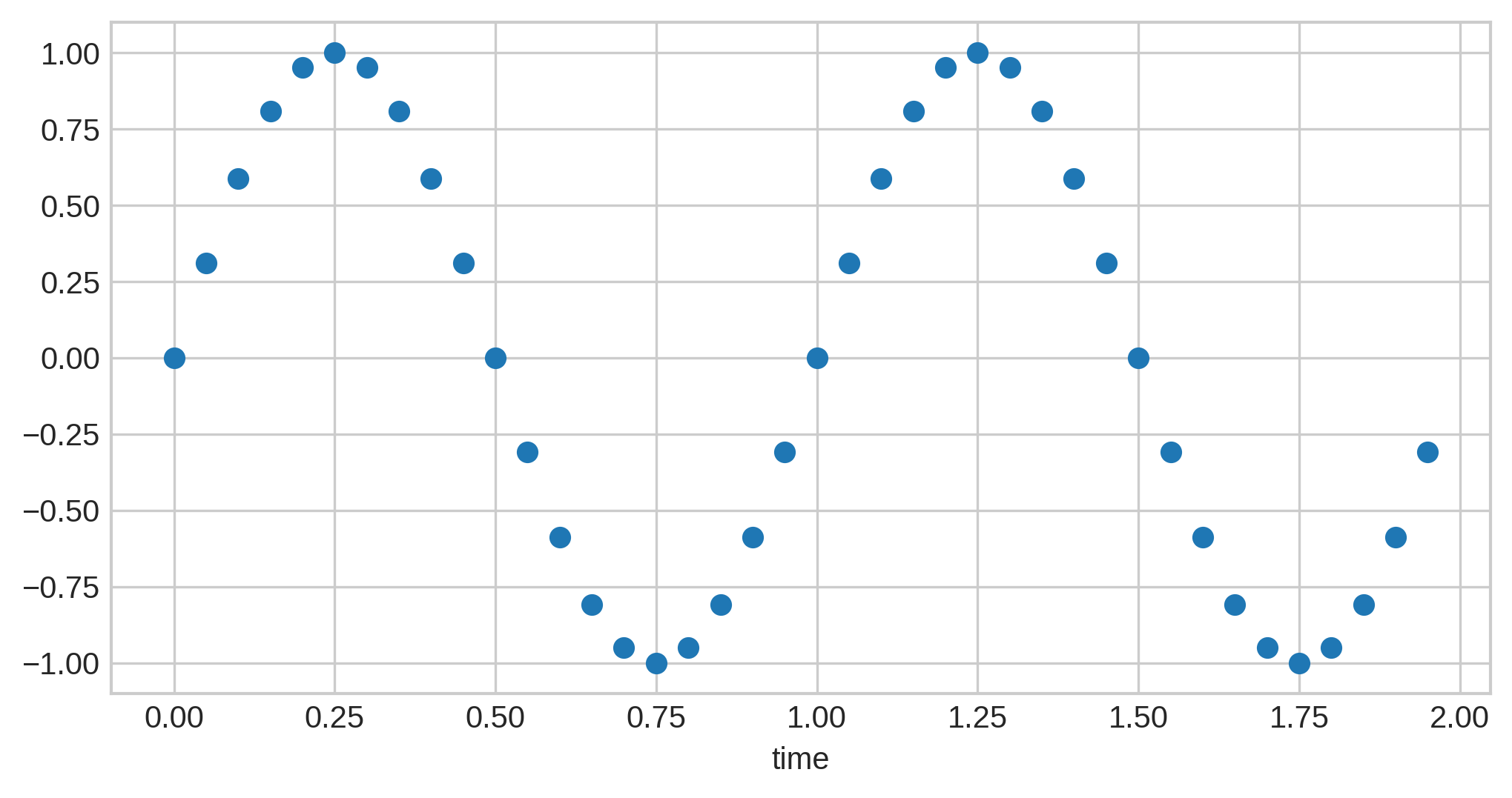
Sound waves themselves are continuous, not discrete, and can be described as an analog signal. (Note: I am aware the definition of "analog" is not exactly this, but for the purposes of our discussion, it’s a "close enough" approximation.) Here’s a very simple sound wave:
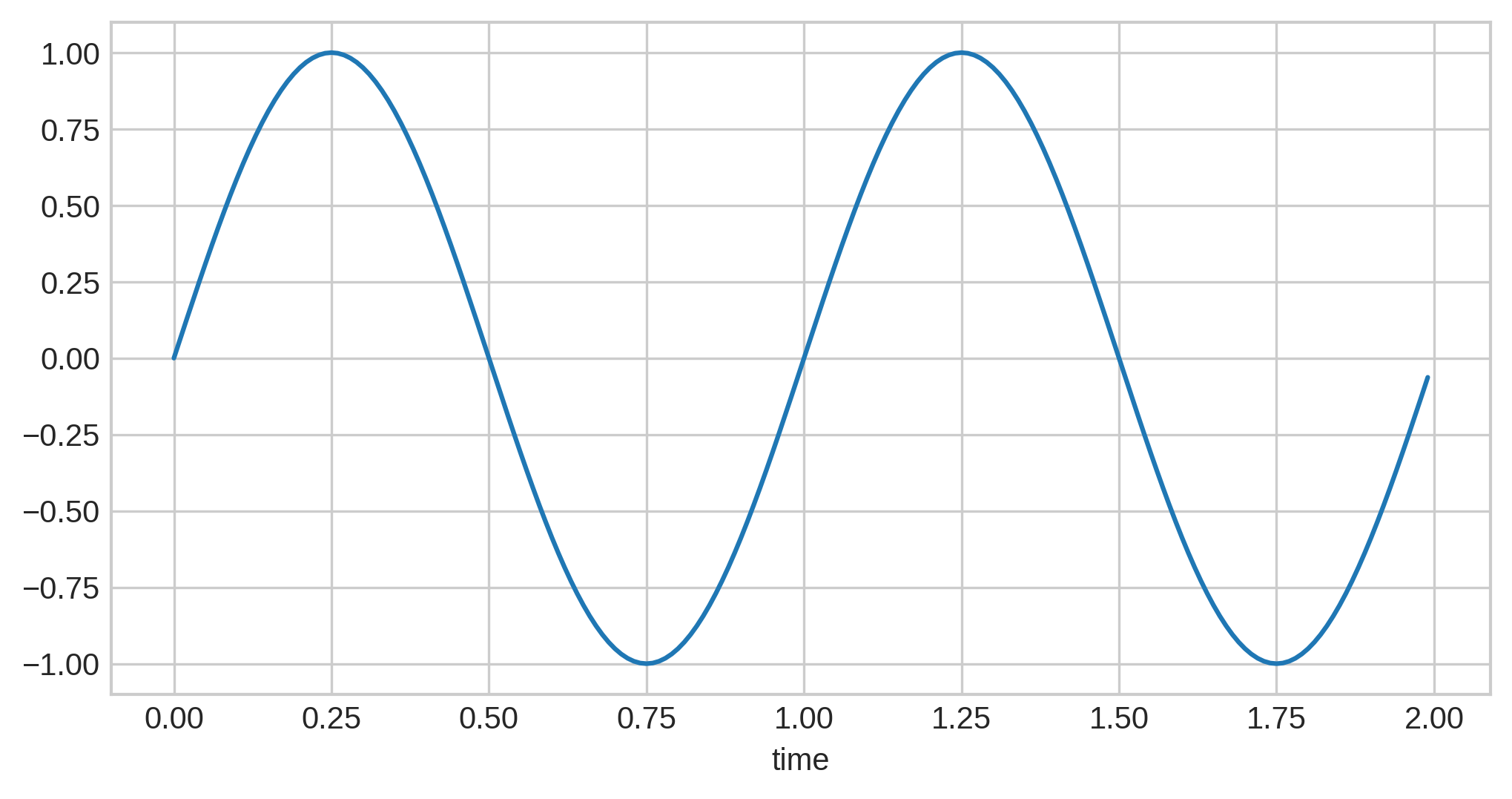
Of course, realistic sound waves are much, much more complex, without the clean repetition seen here.
Unfortunately, this representation poses a problem: how do we store it digitally? Digital signals consist of binary data points (1 or 0), meaning that persisting the infinite number of data points represented by a continuous line is not an option.
Pulse Code Modulation
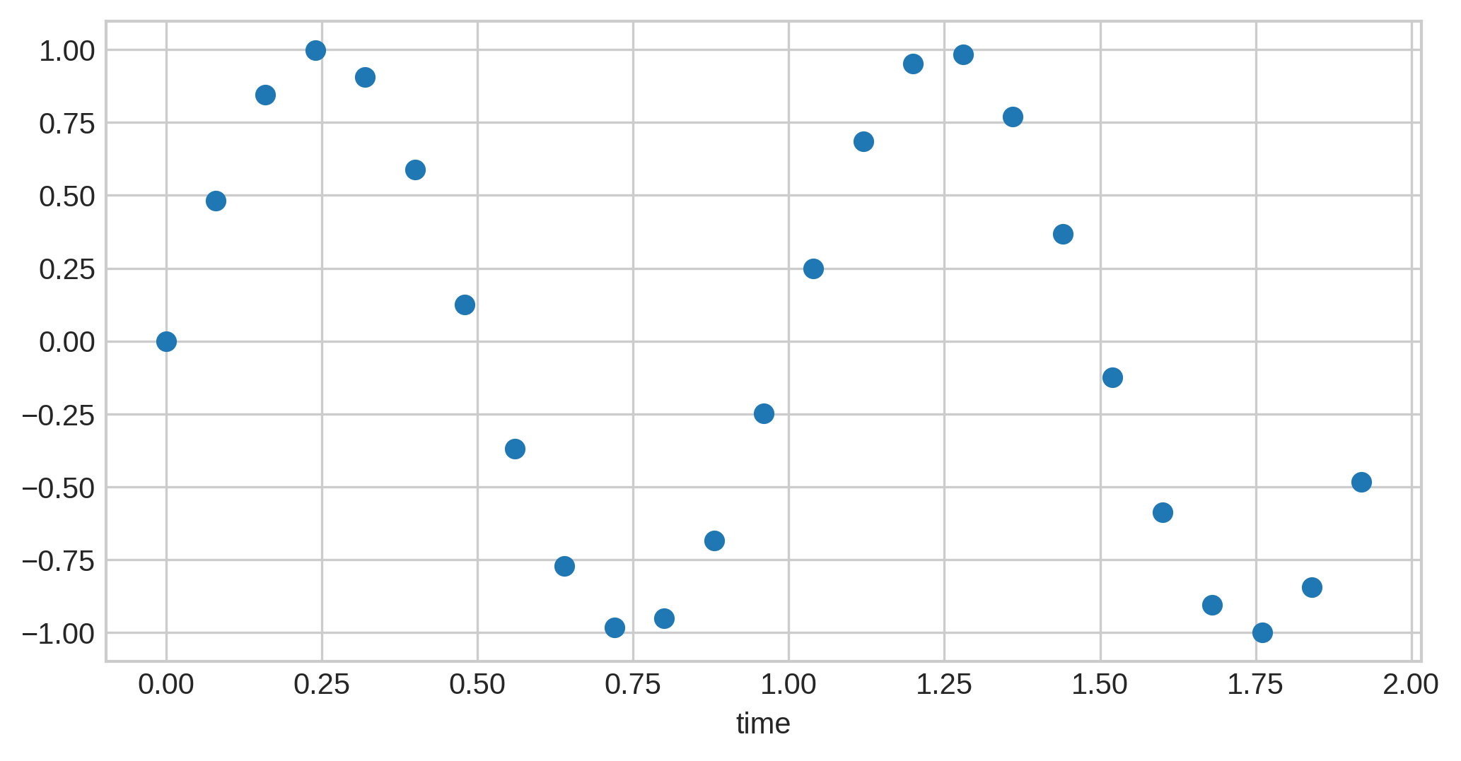
The solution to this problem is simple: we can repeatedly "sample" the value of the continuous line at some point in time and store it as a discrete data point. Here’s what happens if we sample the above audio wave 20 times:
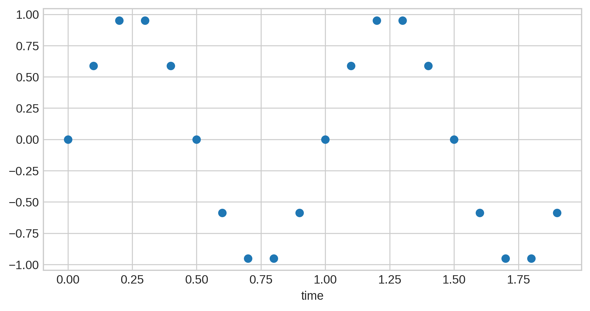
This technique is known as pulse code modulation, or just PCM. (Technically, this is a particular variant of PCM known as linear PCM; discussion of other variants are beyond the scope of this post, though it is worth noting that they are actively used in telephone systems.)
The amount of times audio data is sampled per second is known as its sample rate and is usually measured in kilohertz / KHz, which is thousand of times per second. In other words, a sample rate of 48 KHz means that 48,000 samples are taken per second.
Low sample rates tend to lose more of the original details. If we re-take the above sound wave and sample it 40 times, more details of the curves of preserved:

Now if we increase it by another 20 samples to 60, we get even more detail…but the difference isn’t as high:
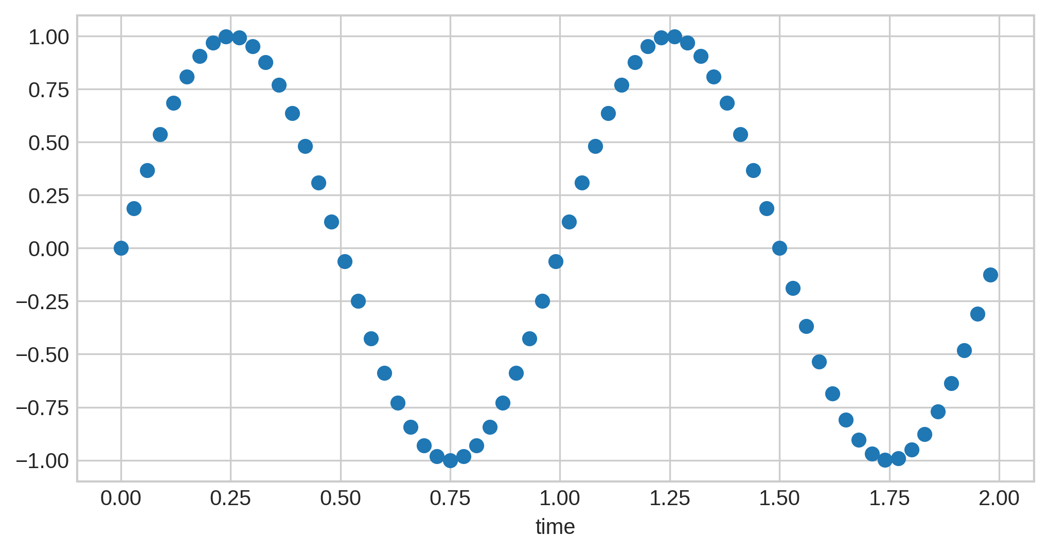
You can see that, although more detail is preserved, it doesn’t add that much; the curves themselves were already visible, and if you were to attempt to retrace the original wave from these discrete points, 60 would not give a noticeably better result than 40.
These same principles apply to realistic audio as well. Standard sample rates tend to hover around the 40-50 KHz range. Just half of that (20 KHz) will sound distinctly worse to many people, but doubling it (~80 KHz) will not sound significantly better to the majority. In other words, increasing sample rates most definitely follow a rule of diminishing returns.
Sample Formats
Now we have a way to represent our continuous audio discretely, but how do we map this to digital storage? In other words, how are these discrete data points actually saved?
There are two primary approaches:
Fixed Point
The most common representation is known as fixed-point, where the data points can be represented as integers along some range. As an example, consider a range of -100 to 100. Our sine wave from above could be represented as:
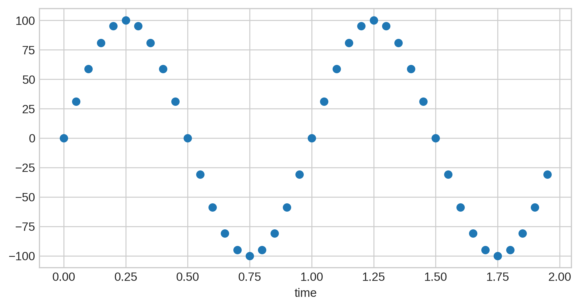
Note the scale on the left: all the audio samples are now in the range we specified, and these values are the ones stored in the PCM data.
In general, the ranges chosen will correspond to the minimum and maximum integers that can be stored in a set number of bits. Exact integer representations are beyond the scope of this post, but the following facts should suffice:
-
The standard method of representing signed integers in computers is known as two’s complement.
-
The largest integer value that can be stored in
kbits via two’s complement representation is2^(k-1)-1. -
The smallest value is
-2^(k-1).
For example, let’s say we want each sample to take up 24 bits of storage. This means that
the lower end of our range will be -2^(24-1) = -8388608, and the upper end of the range
will be 2^(24-1)-1 = 8388607.
There is an exception to this rule: 8-bit fixed-point audio is stored unsigned instead
of signed, meaning that none of the values can be negative. When storing unsigned
integers, two’s complement is not used, and thus the range changes to a minimum of 0 and
a maximum of 2^k-1. Thus, for 8-bit fixed point audio, the minimum end of the range is
0, and the maximum is 2^8-1 = 255.
Floating Point
What if we want even more precision? Instead of having to convert the sample values to
integers, we can convert them to decimals, with 1 as the maximum and -1 as the
minimum, like so:
The format used to store these values is known as IEEE 754 floating point. Although the exact details of this are beyond the scope of this article, one aspect of it is worth noting, that being precision. Even with floats, we still cannot have infinite precision, since, as mentioned above, all digital storage is finite. Thus, the precision used is dependent on the number of bits taken, which according to IEEE 754 is going to be one of 32 or 64 bits (referred to as single precision and double precision, respectively).
Bit Depth and Bitrate
In each of the above representations, we needed a certain number of bits per sample. This value is known as the bit depth. Higher bit depths mean that the ranges are more precise, so the audio data will more accurately be represented. Most audio you hear will have a bit depth of one of the following:
-
8 bits for unsigned fixed point samples
-
16, 24, or 32 bits for signed fixed point samples
-
32 (single-precision) or 64 bits (double-precision) for floating point samples
We can use this information to calculate another metric used to describe audio data,
bitrate, which is essentially the average number of bits used to store some duration of
audio, usually measured in kilobits per second (kbps). This is calculated as
bits-per-sample * sample-rate * audio-channels. For stereo (2-channel) audio with a
24-bit fixed-point sample format and a sample rate of 48KHz will have a bitrate of
2304 kbps.
Resampling and Audio Quality
You can resample audio data to increase or decrease the sample rate and/or change the sample format. However, this can result in permanent degradation of quality. Let’s go back to our audio wave with 20 samples:
Now, say we want to resample this to have 25 samples. You might expect it to look like this:
Ideally, this would be the end result of resampling. However, notice something about the two graphs: the latter has sample points in locations the former did not. For instance, at the peaks of the wave, the one with 25 samples has a point, but the one with 20 samples does not. This means, that if attempting to resample from 20 samples to 25, we would need to insert a sample where it did not previously exist. When this audio data was originally sampled, whatever was at this point was permanently lost, and thus, the best we can now do is use the surrounding audio samples to estimate. The heuristics used to perform these estimations vary in quality, ranging from linear interpolation (simply bases the new sample on the difference between the values of the two surrounding samples) to methods based on a concept known as fourier transforms.
The most important lesson is that resampling audio to a higher sample rate will not restore data that was lost at sampling time. In addition, the same problems apply if going from 25 samples to 20; this also means that resampling audio from sample rate X to Y and then back to X may not result in the original audio data. In other words, resampling can also permanently lose audio data that was present in the original sampled audio.
(Note that there are some exceptions to this: in particular, resampling from sample rate S
to S * N where N is a multiple of 2 will not discard any of the original audio data,
though of course the newly added samples may still not be entirely correct. It is an
exercise to the reader to observe why that is the case; see the 20 vs 40 vs 60 sample rate
graphs above as a reference.)
This logic also applies to changing the sample format.
Intermission: Bitrate and Audio Quality
The above section described one reason why sample rate and format are not sole indicators of audio quality. If you include codecs that compress audio data, however, things get significantly more interesting. In particular, because different codecs have different methods for compressing audio, it is entirely possible that one codec may result in audio files with a lower bitrate but better sound quality than other files. For instance, compare 16kbps Opus with 24kbps MP3. The Opus is audibly significantly clearer, despite the lower bitrate. In addition, some lossy codecs are better at discarding audio data that is not easily audible by the human ear or on most listening setups.
Moral of the story: bitrate should only be used, at best, as an incredibly rough metric of audio quality. A music file with a bitrate of 6kbps is not going to sound particularly excellent regardless of the codec, but a 128kbps file in one codec is not guaranteed to audibly sound any worse than a 192kbps file from another codec, and it’s entirely possible to have a 320kbps audio file that was resampled from a 2kbps file.
WAV Files
Thus far, we have discussed:
-
Continuous and discrete data
-
Converting continuous audio data into discrete points that can be stored digitally
-
Various formats for storing audio data
As well as the following terms:
-
Samples: the individual, discrete data points "sampled" from a continuous audio wave
-
Sample rate: the number of samples taken per second
-
Bit depth: the number of bits required to store audio per second
With this in mind, we can finally start to break down WAV files themselves.
The most interesting thing about a WAV file is that it is technically a "container" that can store multiple different types of audio formats within, but it is rarely used for anything other than PCM data. In addition, WAV itself is a derivative of the RIFF format, developed by Microsoft and IBM. RIFF specifies a format for storing data split into some "chunks", and WAV adds information on top of it for the storage of audio data.
As interesting as that sounds, WAV files in practice are quite simplistic, containing just two RIFF chunks:
-
An "fmt" chunk describing the sound format.
-
A "data" chunk, containing the number of audio samples and the actual audio data.
It may seem odd that the majority of the post was dedicated to everything other than the WAV format itself. WAV is, in fact, an incredibly simple audio format, and this simplicity is what has led to its widespread use, and the stark majority of the logic that goes into audio storage occurs in the PCM realm.
Addendum: Other Audio Formats
WAV is, of course, not the only audio file format. Although a deep dive into other audio formats is well beyond the scope of this article, it may be useful to gain at least a surface level understanding.
First off, there is often a distinction between the form of audio storage and the file that the audio data is in. The mechanism used to encode some audio data is generally referred to as a codec, whereas the file containing the audio data, as well as any other metadata (such as music tags), is referred to as a container. Note that these terms are generally not used entirely consistently, and in many cases, both are referred to together as just the format.
Formats and codecs are generally split into two categories: lossless (stores the entire original audio data) and lossy (discards audio data that is deemed less important to save space). Even with lossless formats, the audio data can still be compressed using various algorithms. For instance, you may have heard of FLAC, one of the most popular lossless audio formats (the standard has both a codec and a container). FLAC is able to achieve a smaller audio size by attempting to match the audio data to a line, which can be stored using far less space than the individual data. Thus, only the differences from the line to the data points need to be stored, resulting in less space usage while preserving the original audio data.
On the lossy end, you’re likely familiar with MP3, AAC, and Ogg Vorbis. This is where the container vs codec distinction begins to show cracks:
-
MP3 generally uses an MPEG-1 container. However, this does not support storing metadata, and a separate format known as ID3 has to be used and stored within the same file.
-
AAC’s container format of choice is MPEG-4 Part 14 (known as just "MP4"). The MP4 container, however, can also store lossless formats (Apple’s ALAC) and even videos (H.264 is commonly used).
-
Ogg itself is actually a generic container format, and it can store other codecs as well, including FLAC. The successor to Vorbis, Opus, also uses an Ogg container, but the file extension was changed for clarity.
Closing Notes
Although this article is already a bit long, it barely scratches the surface of the full world of digital audio. That being said, I hope it can serve as a brief introduction and explanation of some of the terms and concepts you may have heard.